Big-O Notation Quick Reference for Interviews
During a high-stakes technical interview, few moments freeze candidates faster than the inevitable follow-up question: "What is the time and space complexity of your solution, and how would you optimize it?"
Even skilled engineers who write clean, idiomatic code daily can stumble when translating loops, recursive frames, and auxiliary allocations into asymptotic bounds under pressure. Big-O notation is not merely academic theory—it serves as the universal shorthand interviewers use to evaluate your architectural instincts and whether your code can scale from a prototype dataset of 50 items to a distributed pipeline handling 50 million transactions.
This big o notation quick reference provides a battle-tested reference guide designed specifically for interview conditions. We break down the complexity hierarchy, examine side-by-side operation costs across fundamental data structures, analyze standard sorting and searching routines, and outline practical rules to analyze algorithms on a virtual whiteboard.
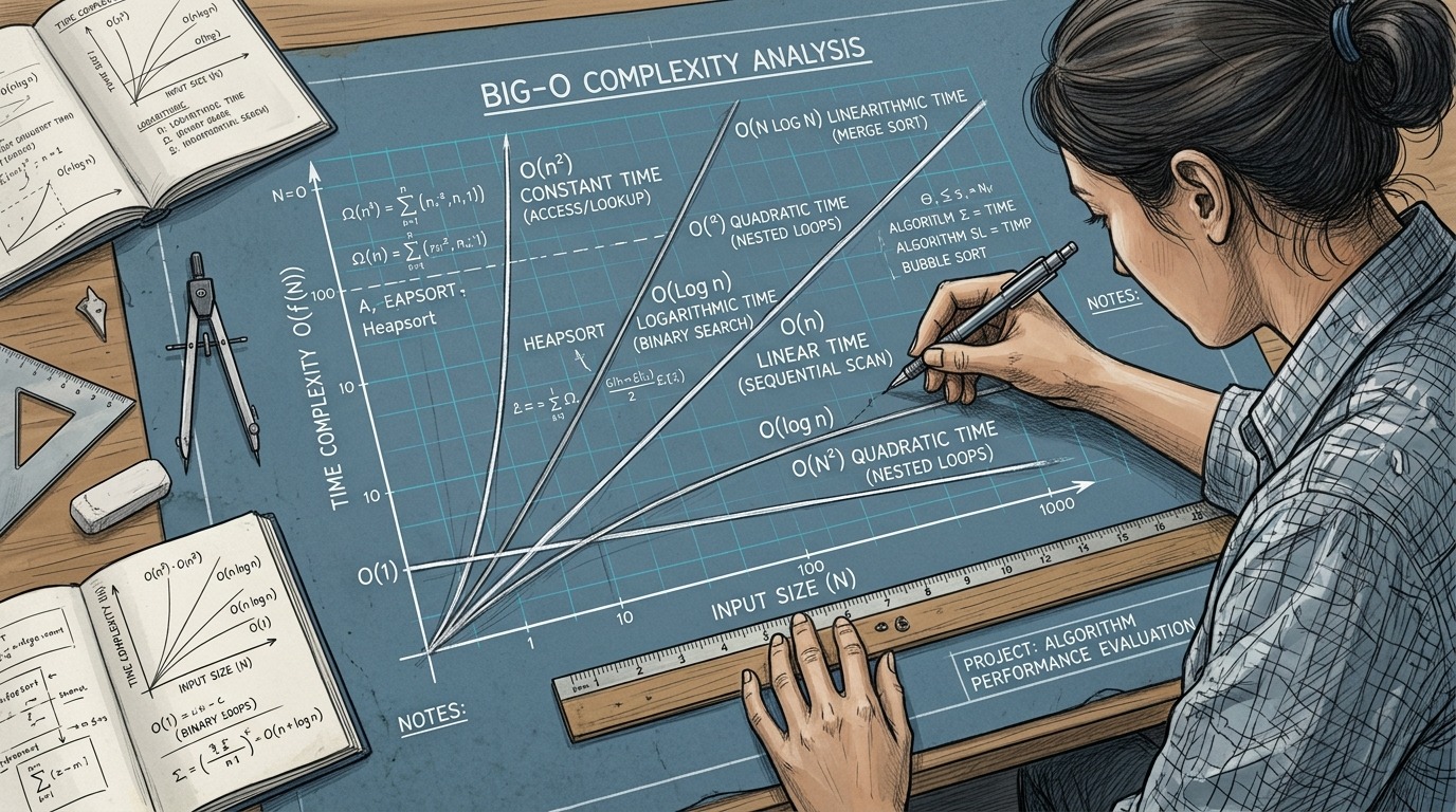
The Big-O Complexity Hierarchy at a Glance
Big-O measures the upper bound of growth: how execution time or memory footprint scales relative to the input size ($n$). When evaluating candidate solutions during a comprehensive technical interview preparation cycle, interviewers categorize performance into clear tiers:
| Notation | Common Name | Relative Speed | Typical Examples |
|---|---|---|---|
| $O(1)$ | Constant | Instantaneous | Hash table key lookup, array indexing by position, stack push/pop |
| $O(\log n)$ | Logarithmic | Extremely Fast | Binary search in a sorted array, balanced search tree lookup |
| $O(n)$ | Linear | Fast | Single loop traversing an array, string scan, linear search |
| $O(n \log n)$ | Linearithmic / Superlinear | Standard for Sorting | Merge sort, Heapsort, average-case Quicksort |
| $O(n^2)$ | Quadratic | Slow for Large Inputs | Nested loops over the same input, Bubble sort, naive duplicate detection |
| $O(n^3)$ | Cubic | Very Slow | Triple nested loops, naive matrix multiplication |
| $O(2^n)$ | Exponential | Impractical for $n > 30$ | Recursive Fibonacci without memoization, generating power sets |
| $O(n!)$ | Factorial | Unusable for $n > 12$ | Generating all permutations via brute force, Travelling Salesperson problem |
Rapid Rule of Thumb
- If an algorithm halves the search space at each iteration, it runs in $O(\log n)$.
- If an algorithm touches every item once, it runs in $O(n)$.
- If an algorithm divides the problem into halves and does linear work per level, it runs in $O(n \log n)$.
- If an algorithm executes nested iterations over the same collection, expect $O(n^2)$.
- If an algorithm doubles its operations for every added input element, it enters $O(2^n)$.
For deep dives into fundamental implementations, compare our companion guide on the Big-O notation cheat sheet for common algorithms or test your knowledge with our data structure interview questions cheat sheet.
Data Structure Operations Reference Matrix
In technical interviews, choosing the appropriate container determines whether an algorithm succeeds in sub-millisecond time or exhausts memory limits. The blueprint below contrasts average and worst-case performance across core structures.
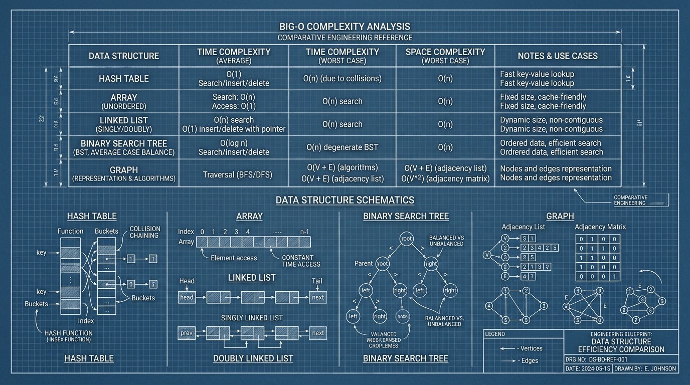
Core Data Structure Operation Complexities
| Data Structure | Access | Search | Insertion | Deletion | Worst-Case Space |
|---|---|---|---|---|---|
| Array (Static) | $O(1)$ | $O(n)$ | $O(n)$ | $O(n)$ | $O(n)$ |
| Dynamic Array (List / Vector) | $O(1)$ | $O(n)$ | $O(1)$ amortized | $O(n)$ | $O(n)$ |
| Singly Linked List | $O(n)$ | $O(n)$ | $O(1)$ at head | $O(1)$ at head | $O(n)$ |
| Doubly Linked List | $O(n)$ | $O(n)$ | $O(1)$ at head/tail | $O(1)$ with node ref | $O(n)$ |
| Stack (LIFO) | $O(n)$ | $O(n)$ | $O(1)$ push | $O(1)$ pop | $O(n)$ |
| Queue (FIFO) | $O(n)$ | $O(n)$ | $O(1)$ enqueue | $O(1)$ dequeue | $O(n)$ |
| Hash Table (Map / Set) | $N/A$ | $O(1)$ avg / $O(n)$ worst | $O(1)$ avg / $O(n)$ worst | $O(1)$ avg / $O(n)$ worst | $O(n)$ |
| Binary Search Tree (Unbalanced) | $O(n)$ | $O(n)$ | $O(n)$ | $O(n)$ | $O(n)$ |
| Balanced BST (AVL / Red-Black) | $O(\log n)$ | $O(\log n)$ | $O(\log n)$ | $O(\log n)$ | $O(n)$ |
| Binary Heap (Min / Max) | $O(1)$ peek min/max | $O(n)$ search | $O(\log n)$ push | $O(\log n)$ pop min/max | $O(n)$ |
Critical Interview Caveats
- Dynamic Array Appends: Appending to a dynamic array (Python
list, JavaArrayList, JavaScriptArray) is $O(1)$ amortized, not absolute $O(1)$. When internal capacity is exceeded, the array allocates double capacity and copies all $n$ items, incurring an occasional $O(n)$ resize penalty. - Hash Table Worst Case: While average lookup is $O(1)$, malicious keys or flawed hash functions cause collisions that degrade hash lookups into $O(n)$ linked list scans or $O(\log n)$ balanced tree buckets. Review our guide on understanding hash tables and collision strategies to handle follow-up system design questions.
- Binary Search Tree Degeneration: Inserting sorted keys into an unaugmented BST produces an asymmetric linked list, degrading search from $O(\log n)$ into $O(n)$. Review binary search tree implementation and edge cases to explain self-balancing rotations.
Searching and Sorting Algorithm Complexities
Interviewers frequently ask candidates to sort inputs before searching or deduplication. Memorize these standard complexities and their memory implications:
Comparison-Based Sorting
| Algorithm | Best Time | Average Time | Worst Time | Auxiliary Space | Stability |
|---|---|---|---|---|---|
| Quicksort | $O(n \log n)$ | $O(n \log n)$ | $O(n^2)$ (poor pivot) | $O(\log n)$ stack | Unstable |
| Merge Sort | $O(n \log n)$ | $O(n \log n)$ | $O(n \log n)$ | $O(n)$ buffers | Stable |
| Heapsort | $O(n \log n)$ | $O(n \log n)$ | $O(n \log n)$ | $O(1)$ in-place | Unstable |
| Insertion Sort | $O(n)$ (nearly sorted) | $O(n^2)$ | $O(n^2)$ | $O(1)$ | Stable |
| Selection Sort | $O(n^2)$ | $O(n^2)$ | $O(n^2)$ | $O(1)$ | Unstable |
| Timsort (Python / JS default) | $O(n)$ | $O(n \log n)$ | $O(n \log n)$ | $O(n)$ | Stable |
For step-by-step visual comparisons of execution routines, inspect top 10 sorting algorithms visualized.
Graph & Tree Traversal Complexities
| Algorithm | Graph Representation | Time Complexity | Auxiliary Space Complexity |
|---|---|---|---|
| Breadth-First Search (BFS) | Adjacency List | $O(V + E)$ | $O(V)$ queue + visited set |
| Depth-First Search (DFS) | Adjacency List | $O(V + E)$ | $O(V)$ call stack + visited set |
| Dijkstra's Shortest Path | Min-Heap + Adjacency List | $O((V + E) \log V)$ | $O(V)$ distance map + heap |
| Topological Sort (Kahn's) | In-Degree Map + Queue | $O(V + E)$ | $O(V)$ |
$V$ represents the number of vertices; $E$ represents the number of edges.
Space vs. Time Complexity Trade-Offs
In competitive coding and real-world system architecture, engineers rarely obtain speed improvements without consuming auxiliary memory.
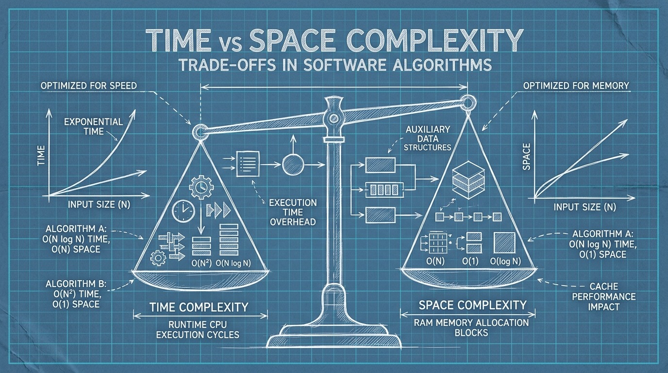
Auxiliary Space vs. Total Space
Candidates often confuse auxiliary space with input space:
- Total Space: Input data storage ($O(n)$ for an array of length $n$) plus any temporary allocations.
- Auxiliary Space: Only the extra or temporary storage your algorithm creates to solve the problem (excluding the input arguments).
When interviewers say "Can you do this in $O(1)$ space?", they mean $O(1)$ auxiliary space—modifying the input array in-place or utilizing pointers rather than allocating auxiliary hash sets or cloned collections.
The Three Classic Trade-Off Patterns
- Hash Map Caching (Time $O(n^2) \rightarrow O(n)$, Space $O(1) \rightarrow O(n)$): Instead of checking all pairs with two nested loops ($O(n^2)$ time), store seen elements in a hash map to look up complementary keys in $O(1)$ average time.
- In-Place Two-Pointer Modification (Time $O(n)$, Space $O(n) \rightarrow O(1)$): Instead of filtering elements into a new slice or array, maintain read and write indices to overwrite elements in place without dynamic heap allocations.
- Dynamic Programming Tabulation vs. Memoization: Top-down recursive memoization requires $O(n)$ stack frames plus $O(n)$ cache entries. Bottom-up iterative tabulation can frequently reduce auxiliary space to $O(1)$ by retaining only the previous two computed states (as seen in Fibonacci or climbing stairs).
4 Practical Rules to Calculate Big-O Under Pressure
When calculating algorithmic bounds during a live coding interview on totop.app, apply these systematic evaluation steps:
Rule 1: Drop Constants and Non-Dominant Terms
Big-O describes asymptotic behavior as $n \to \infty$. Constant multipliers and smaller growth factors disappear: $O(3n^2 + 500n + 12000) \implies O(n^2)$ $O(n + \log n) \implies O(n)$
def process_data(items):
    # Phase 1: O(n)
    for x in items:
        print(x)

    # Phase 2: O(n^2)
    for i in range(len(items)):
        for j in range(len(items)):
            compute_pair(items[i], items[j])

# Total: O(n + n^2) -> Dominant term is O(n^2)
Rule 2: Distinguish Between Multiple Independent Inputs
Never combine independent inputs into a single variable $n$. If your function accepts two arrays A and B of lengths $a$ and $b$:
# Sequential iterations: O(a + b)
def iterate_both(arr_a, arr_b):
    for item in arr_a:  # O(a)
        do_work(item)
    for item in arr_b:  # O(b)
        do_work(item)

# Nested iterations: O(a * b)
def cross_product(arr_a, arr_b):
    for x in arr_a:      # a iterations
        for y in arr_b:  # b iterations
            compare(x, y)
Stating that cross_product runs in $O(n^2)$ is technically inaccurate; the correct answer is $O(a \cdot b)$. Stating the precise variables demonstrates seasoned engineering rigour.
Rule 3: Recursive Branching Factor Formula
For recursive algorithms without memoization, compute complexity using the branch-and-depth formula: $\text{Time Complexity} = O(\text{Branches}^{\text{Depth}})$ $\text{Space Complexity} = O(\text{Maximum Call Stack Depth})$
In a naive Fibonacci implementation:
def fib(n):
    if n <= 1:
        return n
    return fib(n - 1) + fib(n - 2)
- Each call branches into 2 calls.
- The tree reaches a maximum depth of $n$.
- Time Complexity: $O(2^n)$.
- Auxiliary Space: $O(n)$ due to the activation frames stored on the call stack.
Rule 4: Watch for Costly String and Array Built-Ins
Language built-ins frequently hide linear work beneath clean syntax:
- In Python,
array.pop(0)is $O(n)$ because remaining elements shift left. Usecollections.dequefor $O(1)$ pop left operations. - In JavaScript,
Array.prototype.unshift()andArray.prototype.shift()are $O(n)$. - String concatenation inside loops (
s += char) in languages with immutable strings (Java, Python, C#) generates a new string object each time, turning an apparently $O(n)$ loop into $O(n^2)$. UseStringBuilderor''.join(list).
Candidates struggling with time constraints often find our actionable strategies on how to pass coding interviews without LeetCode grinding helpful for identifying high-leverage conceptual patterns over rote memorization.
Rehearsing Complexity Explanations for Your Interview
Knowing the correct Big-O value is only half the battle—articulating your reasoning clearly to an interviewer completes the assessment.
Follow this 3-step verbal formula:
- State the Time Complexity First: "The solution runs in $O(n \log n)$ time because sorting the array takes $O(n \log n)$, followed by a single linear scan of $O(n)$."
- State the Space Complexity Second: "The auxiliary space complexity is $O(1)$ because we mutate the pointers directly without allocating supplementary buffers or recursion frames."
- Acknowledge Edge Cases or Amortized Costs: "On average, the hash table lookup is $O(1)$, but in the worst case with excessive hash collisions, it can degrade to $O(n)$."
To build fluid muscle memory before sitting across from a real hiring manager, simulate realistic mock interviews on totop.app. With customizable technical questions and instant AI feedback on code efficiency and complexity justifications, you can transform Big-O analysis from a point of anxiety into your competitive advantage.