Data Structure Interview Questions Cheat Sheet
Technical interviews rarely evaluate whether you have memorized a textbook definition of an AVL tree or a doubly linked list. Instead, interviewers evaluate your ability to select, defend, and implement the optimal data structure under strict algorithmic constraints, memory limits, and hardware realities.
When an interviewer asks you to solve a problem like finding the running median of an incoming stream of integers or identifying the earliest duplicate timestamp in a distributed log, your choice of data structure dictates your solution's asymptotic bounds. Selecting a linked list when you need random access adds an accidental $O(n)$ penalty to every iteration. Conversely, choosing an array without considering resizing costs can turn a smooth sub-millisecond pipeline into a jittery latency bottleneck.
This data structure interview questions cheat sheet consolidates the operational mechanics, Big-O bounds, architectural trade-offs, and high-frequency interview patterns across all fundamental data structures. Bookmark this guide to review before your upcoming coding screens and whiteboard rounds.
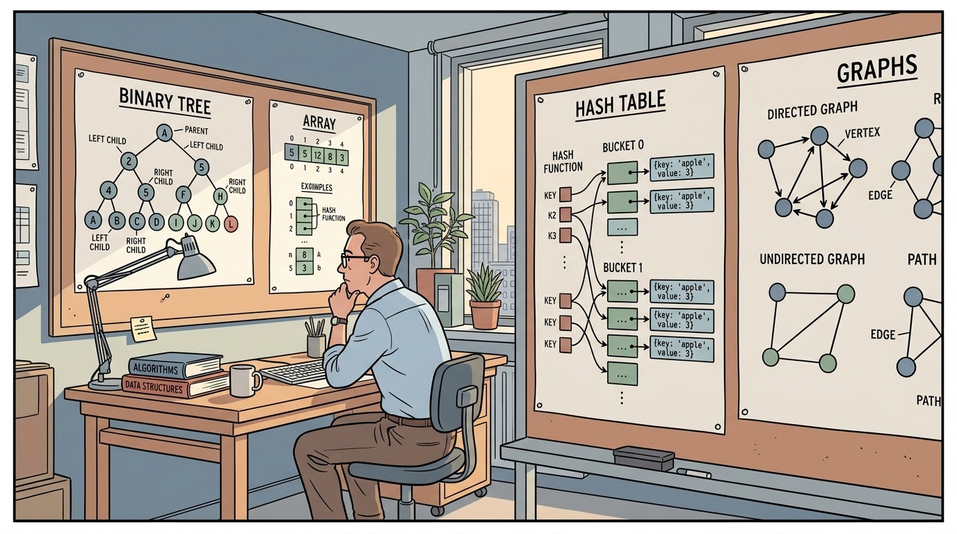
1. Master Data Structure Complexity Matrix
Before examining individual structures, use this master matrix to compare average and worst-case time complexities alongside auxiliary space requirements. For detailed background on growth curves and asymptotic proofs, consult our Big-O notation quick reference for interviews.
| Data Structure | Access (Avg / Worst) | Search (Avg / Worst) | Insertion (Avg / Worst) | Deletion (Avg / Worst) | Space (Worst) | Primary Use Case |
|---|---|---|---|---|---|---|
| Array | $O(1) / O(1)$ | $O(n) / O(n)$ | $O(n) / O(n)$ | $O(n) / O(n)$ | $O(n)$ | Constant-time random access by index; fixed-size lookup tables |
| Dynamic Array | $O(1) / O(1)$ | $O(n) / O(n)$ | $O(1)^am / O(n)$ | $O(n) / O(n)$ | $O(n)$ | Resizable collections, sequential scans, fast cache iteration |
| Singly Linked List | $O(n) / O(n)$ | $O(n) / O(n)$ | $O(1) / O(1)$* | $O(1) / O(1)$* | $O(n)$ | Frequent head insertions/deletions, queue implementations |
| Doubly Linked List | $O(n) / O(n)$ | $O(n) / O(n)$ | $O(1) / O(1)$* | $O(1) / O(1)$* | $O(n)$ | LRU Cache implementation, bidirectional navigation |
| Stack (LIFO) | $O(n) / O(n)$ | $O(n) / O(n)$ | $O(1) / O(1)$ | $O(1) / O(1)$ | $O(n)$ | Expression parsing, undo mechanisms, DFS recursion tracking |
| Queue (FIFO) | $O(n) / O(n)$ | $O(n) / O(n)$ | $O(1) / O(1)$ | $O(1) / O(1)$ | $O(n)$ | Task scheduling, Breadth-First Search (BFS), buffering |
| Hash Table / Map | N/A | $O(1) / O(n)$ | $O(1) / O(n)$ | $O(1) / O(n)$ | $O(n)$ | Key-value mapping, $O(1)$ presence checks, frequency counting |
| Binary Search Tree | $O(\log n) / O(n)$ | $O(\log n) / O(n)$ | $O(\log n) / O(n)$ | $O(\log n) / O(n)$ | $O(n)$ | Ordered data retrieval, range queries, predecessor search |
| Balanced BST (AVL / Red-Black) | $O(\log n) / O(\log n)$ | $O(\log n) / O(\log n)$ | $O(\log n) / O(\log n)$ | $O(\log n) / O(\log n)$ | $O(n)$ | Guaranteed logarithmic operations; language standard maps |
| Binary Heap (Priority Queue) | N/A | $O(n) / O(n)$ | $O(\log n) / O(\log n)$ | $O(\log n) / O(\log n)$** | $O(n)$ | Streaming Top-K elements, Dijkstra's shortest path, event scheduling |
| Trie (Prefix Tree) | N/A | $O(L) / O(L)$ | $O(L) / O(L)$ | $O(L) / O(L)$ | $O(A \cdot L)$ | Autocomplete, prefix matching, spell check ($L$ = length, $A$ = alphabet) |
| Graph (Adjacency List) | N/A | $O(V + E)$ | $O(1)$ | $O(E)$ | $O(V + E)$ | Network relationships, dependency resolution, routing maps |
* Insertion and deletion in linked lists take $O(1)$ time only when you already hold a direct reference/pointer to the node in question. Locating that node first requires an $O(n)$ traversal.
** Deletion in a binary heap refers to extracting the root element (extract-min or extract-max). Deleting an arbitrary element requires $O(n)$ search followed by $O(\log n)$ sift-down.
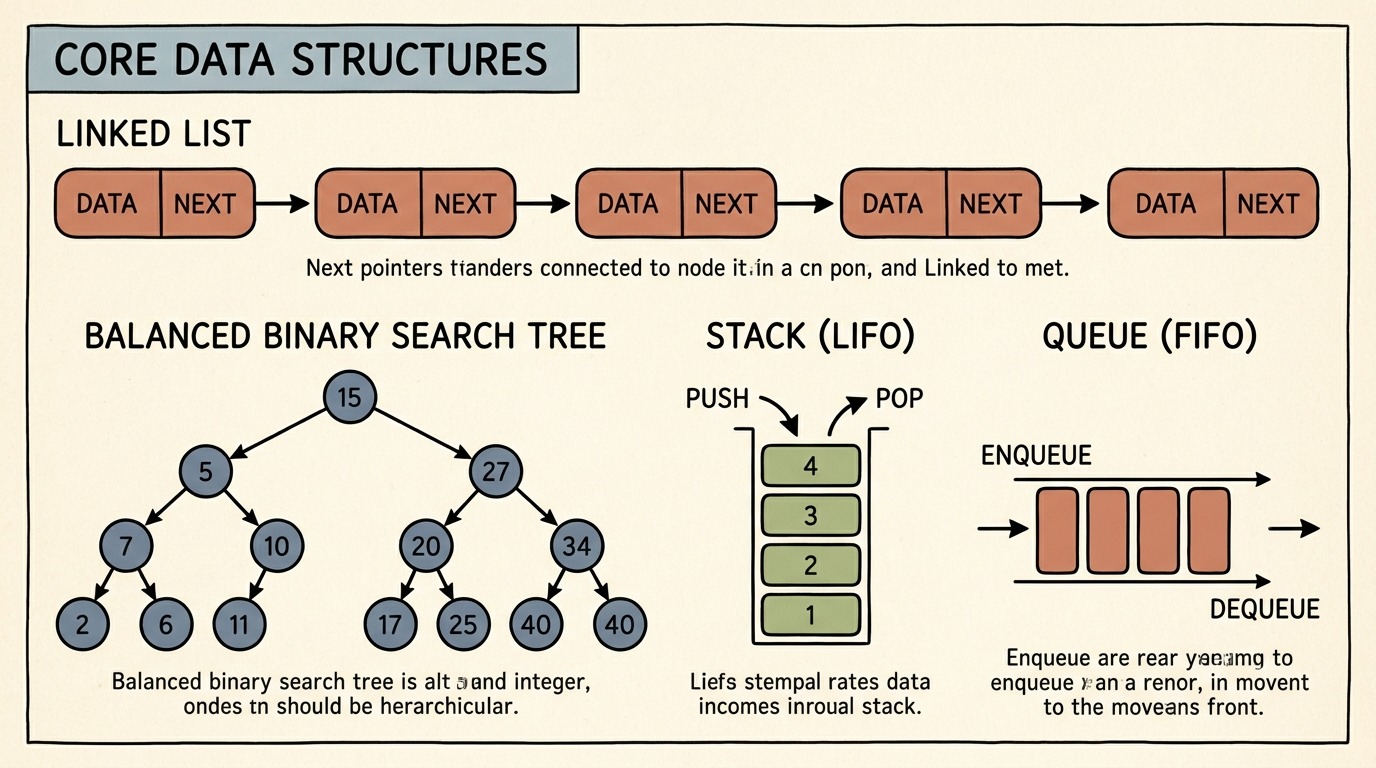
2. Contiguous vs. Pointer-Based Layout: The Hardware Reality
One of the most effective ways to impress a senior or staff engineering interviewer is explaining why theoretical Big-O complexity sometimes diverges from production hardware benchmarks.
In classical algorithm theory, inserting an element at the beginning of a singly linked list is $O(1)$, while inserting into an array is $O(n)$ because every subsequent element must shift right. Yet in modern microprocessors, traversing an array of 10,000 items is often orders of magnitude faster than traversing a linked list of the same length.
Spatial Locality and CPU Cache Lines
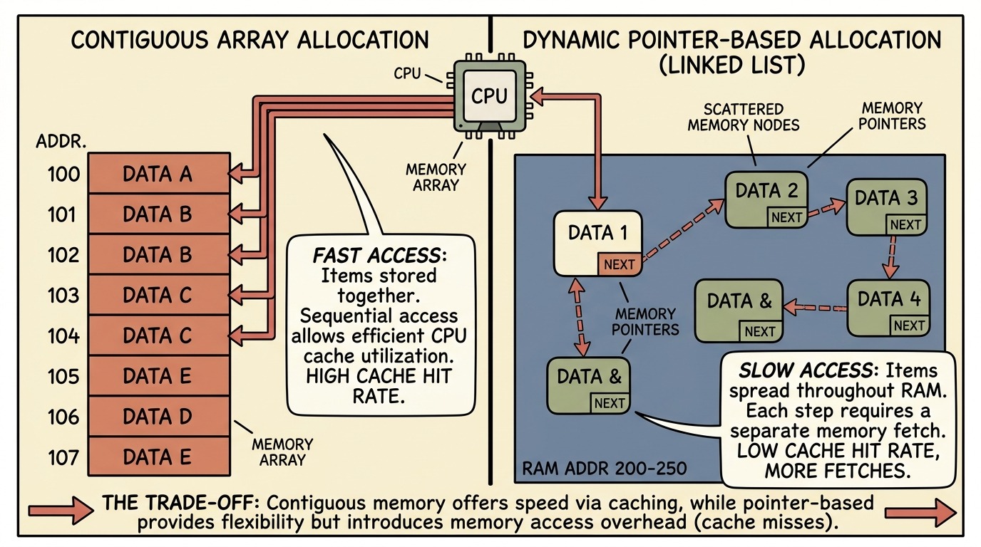
Modern CPUs fetch memory in 64-byte cache lines. When your program reads index arr[0], the CPU pre-fetches contiguous neighboring elements into the ultra-fast L1/L2 data cache. Sequential access over arrays results in near-100% cache hit rates.
In contrast, linked list nodes, tree nodes, and graph vertex objects are allocated independently on the heap. Their memory addresses are fragmented throughout RAM. Every pointer dereference forces the CPU to stall while performing a memory bus round-trip—a phenomenon known as pointer chasing and cache misses.
Interview Pro-Tip: When asked about trade-offs between an array-backed structure and a linked list on a whiteboard, explicitly mention cache locality and memory overhead (e.g., each 64-bit pointer adds 8 bytes of auxiliary overhead per node). This demonstrates system-level thinking beyond pure theoretical asymptotic notation.
3. High-Frequency Interview Questions & Implementation Patterns
Let's dissect the core data structures tested during technical screens, along with their canonical problem archetypes and edge cases.
A. Arrays & Dynamic Arrays (Strings)
An array stores elements in contiguous memory addresses. Dynamic arrays (like Python's list, Java's ArrayList, or C++'s std::vector) allocate a backing static array and automatically double their capacity when full, achieving $O(1)$ amortized insertion.
Common Interview Archetypes
- Two Pointers: Moving inward from opposite ends (e.g., checking palindromes, Container With Most Water, sorting two-color arrays) or tracking fast/slow indices.
- Sliding Window: Maintaining a dynamic contiguous range $[L, R]$ to compute running aggregates (e.g., minimum size subarray sum, longest substring without repeating characters).
- Prefix Sums: Precomputing cumulative totals in $O(n)$ time to answer arbitrary range-sum queries in $O(1)$ time.
Canonical Interview Question: Sliding Window Maximum
from collections import deque

def max_sliding_window(nums: list[int], k: int) -> list[int]:
    """
    Find the maximum value in each sliding window of size k.
    Runs in O(n) time using a monotonic decreasing deque.
    """
    result = []
    window = deque()  # Stores indices of elements in decreasing order

    for i, num in enumerate(nums):
        # 1. Pop indices that are outside the current window
        if window and window[0] <= i - k:
            window.popleft()

        # 2. Maintain monotonic decreasing property
        while window and nums[window[-1]] <= num:
            window.pop()

        window.append(i)

        # 3. Add to result once the first window is fully formed
        if i >= k - 1:
            result.append(nums[window[0]])

    return result
B. Linked Lists (Singly & Doubly)
Linked lists store nodes containing data and one or more address pointers. They excel when fast insertions and deletions occur at known node references or endpoints, without needing contiguous memory allocation.
Common Interview Archetypes
- Fast and Slow Pointers (Floyd’s Cycle-Finding): Detecting loops, finding the cycle entry point, or locating the midpoint of a list in a single pass.
- Sentinel / Dummy Head Nodes: Eliminating messy edge-case handling when inserting or deleting at the list head.
- In-Place Pointer Reversal: Reversing nodes in-place using three pointers (
prev,curr,next) without allocating extra heap memory.
Canonical Interview Question: In-Place Reverse of a Singly Linked List
class ListNode:
    def __init__(self, val=0, next=None):
        self.val = val
        self.next = next

def reverse_list(head: ListNode | None) -> ListNode | None:
    """
    Reverses a singly linked list in-place in O(n) time and O(1) space.
    """
    prev = None
    curr = head

    while curr:
        next_node = curr.next  # Save next node
        curr.next = prev       # Reverse pointer
        prev = curr            # Move prev forward
        curr = next_node       # Move curr forward

    return prev
C. Hash Tables & Hash Sets
Hash tables map keys to values using a mathematical hash function that translates arbitrary keys into array bucket indices. When collisions occur, systems resolve them via chaining (linked lists or balanced trees per bucket) or open addressing (linear or quadratic probing).
For a granular breakdown of collision math, load factors, and cryptographic vs. non-cryptographic hash algorithms, read our deep dive on understanding hash tables collisions and performance.
Common Interview Archetypes
- Frequency Counter: Mapping items to occurrences to detect anagrams, majorities, or duplicates in $O(n)$ time.
- Complement Lookup: Transforming nested $O(n^2)$ pair searches into $O(n)$ single-pass lookups (the core foundation of the classic Two Sum pattern).
- Design Problems (LRU Cache): Combining a hash map for $O(1)$ key lookup with a doubly linked list for $O(1)$ eviction ordering.
Critical Trap: Hash Collision Degradation
If an adversarial dataset causes all keys to collide into the same bucket, lookup complexity degrades from $O(1)$ to $O(n)$ under linked list chaining. Java 8+ mitigates this by converting long bucket lists into red-black trees when bucket depth exceeds 8, capping worst-case lookups at $O(\log n)$.
D. Stacks & Queues
- Stack (LIFO): Elements enter and exit from the top. Essential for depth-first searches, compiler parenthesis validation, and monotonic boundary checks.
- Queue (FIFO): Elements enter at the tail and exit at the head. Fundamental for breadth-first graph explorations and asynchronous message buffering.
Monotonic Stack Pattern
When an interview question asks for the "next greater element," "stock span," or "largest rectangle in a histogram," your immediate instinct should be a monotonic stack. A monotonic stack maintains elements in strictly increasing or decreasing order. By discarding elements that violate the monotonicity, each element enters and leaves the stack at most once, yielding an $O(n)$ total runtime.
def next_greater_element(nums: list[int]) -> list[int]:
    """
    Returns an array where result[i] is the next greater element for nums[i],
    or -1 if no greater element exists. Runs in O(n) time.
    """
    n = len(nums)
    result = [-1] * n
    stack = []  # Stores indices of elements

    for i in range(n):
        while stack and nums[stack[-1]] < nums[i]:
            idx = stack.pop()
            result[idx] = nums[i]
        stack.append(i)

    return result
E. Trees & Binary Search Trees (BST)
Trees model hierarchical relationships. A Binary Search Tree (BST) enforces the invariant: for every node, all values in its left subtree are strictly smaller, and all values in its right subtree are strictly greater.
Traversal Orderings Cheat Sheet
- In-Order (Left, Root, Right): Produces keys in strictly sorted ascending order in a valid BST.
- Pre-Order (Root, Left, Right): Ideal for cloning or serializing tree topologies.
- Post-Order (Left, Right, Root): Crucial for bottom-up evaluations, such as calculating subtree heights, deleting nodes, or verifying BST validity.
- Level-Order (Breadth-First): Uses a FIFO queue to process nodes tier by tier; critical for finding shortest paths in unweighted trees.
To see step-by-step implementations and balanced balancing routines, explore our guide on binary search trees implementation and use cases.
Degenerate Tree Warning
If you insert pre-sorted data into an unbalanced BST without balancing rotations (AVL or Red-Black), the tree devolves into a skewed singly linked list. Operations collapse from $O(\log n)$ to $O(n)$.
F. Heaps & Priority Queues
A binary heap is a complete binary tree backed by a flat contiguous array that satisfies the heap property:
- Min-Heap: The root holds the minimum element; each parent is smaller than or equal to its children (
arr[i] <= arr[2i+1]andarr[i] <= arr[2i+2]). - Max-Heap: The root holds the maximum element.
Array Index Mapping Formulas
- Parent of index
i:(i - 1) // 2 - Left child of index
i:2 * i + 1 - Right child of index
i:2 * i + 2
Top-K Pattern: Choosing Min-Heap vs. Max-Heap
Candidates frequently invert heap types during interviews. Remember this golden rule:
- Finding the Top $K$ Largest elements: Maintain a Min-Heap of fixed size $K$. Every incoming element is compared against the minimum of your top set. If larger, pop the min and push the new item. Time complexity: $O(n \log K)$.
- Finding the Top $K$ Smallest elements: Maintain a Max-Heap of fixed size $K$.
import heapq

def find_kth_largest(nums: list[int], k: int) -> int:
    """
    Returns the k-th largest element using a min-heap of capacity k.
    Runs in O(n log k) time and O(k) auxiliary space.
    """
    heap = []
    for num in nums:
        heapq.heappush(heap, num)
        if len(heap) > k:
            heapq.heappop(heap)
    return heap[0]
Heapify Complexity: Building a heap from an unordered array of $n$ elements using bottom-up sift-down takes $O(n)$ time, not $O(n \log n)$. This mathematical property relies on the converging geometric series $\sum \frac{h}{2^h} = 2$.
G. Graphs & Disjoint Sets (Union-Find)
Graphs model networks consisting of vertices ($V$) connected by edges ($E$). In interviews, graphs appear as adjacency lists, 2D grid mazes, or dependency DAGs (Directed Acyclic Graphs).
For a complete breakdown of traversal algorithms, shortest-path algorithms, and cycle checks, see our companion article on graph algorithms for software engineers.
Representation Trade-offs
- Adjacency Matrix ($V \times V$ boolean grid): $O(1)$ edge existence checks, but consumes $O(V^2)$ memory. Inefficient for sparse real-world graphs.
- Adjacency List (Map of node to neighbors list): Consumes $O(V + E)$ memory; standard choice for BFS and DFS graph interviews.
Union-Find (Disjoint Set Union - DSU)
Used to detect cycles in undirected graphs, compute connected components, and implement Kruskal’s Minimum Spanning Tree. With path compression and union by rank/size, DSU operations run in near-constant $O(\alpha(n))$ amortized time, where $\alpha$ is the Inverse Ackermann function (effectively $\le 4$ for any real-world dataset).
class DSU:
    def __init__(self, size: int):
        self.parent = list(range(size))
        self.rank = [1] * size

    def find(self, x: int) -> int:
        if self.parent[x] != x:
            self.parent[x] = self.find(self.parent[x])  # Path compression
        return self.parent[x]

    def union(self, x: int, y: int) -> bool:
        root_x = self.find(x)
        root_y = self.find(y)
        if root_x == root_y:
            return False  # Already in the same set (cycle detected)

        # Union by rank
        if self.rank[root_x] < self.rank[root_y]:
            self.parent[root_x] = root_y
        elif self.rank[root_x] > self.rank[root_y]:
            self.parent[root_y] = root_x
        else:
            self.parent[root_y] = root_x
            self.rank[root_x] += 1

        return True
H. Tries (Prefix Trees)
A Trie is an $n$-ary tree where edges or nodes represent characters of an alphabet. Common applications include search engine autocomplete suggestions, IP routing tables, and Boggle solvers.
       (root)
      /      \
    'c'      'd'
     |        |
    'a'      'o'
    / \       |
  't' 'r'    'g'
- Search Time: Exactly $O(L)$, where $L$ is the length of the query string. Crucially, search speed is completely independent of the number of words stored in the dictionary ($N$).
- Space Trade-off: Memory consumption can be steep if nodes use fixed 26-pointer arrays. Real-world implementations utilize hash maps or ternary search trees to conserve empty child references.
4. The 5-Step Framework: Picking the Right Data Structure on the Fly
When confronted with an ambiguous coding question in an interview, apply this sequential decision tree:
- Step 1: Clarify Access & Mutation Patterns
- Need direct index access in $O(1)$? $\rightarrow$ Array / Vector.
- Need constant-time insertions/deletions only at ends? $\rightarrow$ Deque / Doubly Linked List.
- Need $O(1)$ key-value associations? $\rightarrow$ Hash Map.
- Step 2: Inspect Ordering Requirements
- Must keys remain in sorted order for range scans or predecessor queries? $\rightarrow$ Balanced Binary Search Tree (Red-Black / AVL) or Skip List.
- Must you process elements by priority rather than arrival? $\rightarrow$ Binary Heap.
- Must you retrieve elements in First-In-First-Out sequence? $\rightarrow$ Queue.
- Step 3: Check Boundary Conditions
- Are you repeatedly querying minimum or maximum boundaries in a sliding sequence? $\rightarrow$ Monotonic Deque or Heap.
- Are you validating nested scopes or matching brackets? $\rightarrow$ Stack.
- Step 4: Check Prefix & Connectivity Requirements
- Searching for shared string prefixes or dictionary lookups? $\rightarrow$ Trie.
- Tracking dynamic cluster connectivity or network partitions? $\rightarrow$ Disjoint Set Union (DSU).
- Searching shortest paths across unweighted states? $\rightarrow$ Breadth-First Search on a Graph.
- Step 5: Synthesize Combined Structures
- Complex interview problems frequently fuse two data structures:
- LRU Cache: Hash Map + Doubly Linked List.
- LFU Cache: Hash Map + Doubly Linked Lists ordered by frequency.
- Median of Running Stream: Two Heaps (Max-Heap for lower half, Min-Heap for upper half).
- Complex interview problems frequently fuse two data structures:
5. Whiteboard Traps and Edge Cases to Mention Proactively
Senior engineers differentiate themselves by identifying edge cases before writing code:
- Empty Collection Guard: Always verify whether input pointers can be
None/nullor empty lists before accessing heads or indices. - Integer Overflow on Binary Search Midpoints: In languages like Java or C++, computing
mid = (low + high) // 2can cause integer overflow when arrays exceed