When I first encountered Big-O notation, it felt like an abstract math puzzle designed to make coding interviews unnecessarily stressful. I still remember staring at complexity charts, trying to memorize why O(log n) was better than O(n), and wondering if I'd ever actually use this in a real job.
But once you strip away the academic jargon, Big-O is just a tool for talking about performance. It’s the language we use to answer one simple question: "How does our code slow down or consume more memory as our data grows?"
Whether you are preparing for a technical interview on totop.app or trying to optimize a sluggish production endpoint, having a clear mental model of time and space complexity is your superpower. For an interview-focused summary and operation matrix, check out our Big-O notation quick reference for interviews and our comprehensive data structure interview questions cheat sheet.
Let’s skip the academic proofs and dive into the practical cheat sheet for the most common complexities and algorithms you will see in the wild.

The Big-O Complexity Hierarchy
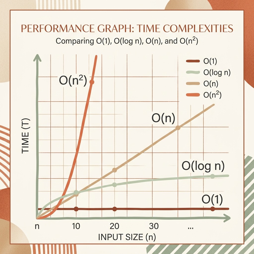
Before looking at the algorithms, let's look at the spectrum of efficiency. We generally group complexities from best to worst:
O(1)— Constant Time: Performance is independent of input size. The holy grail.O(log n)— Logarithmic Time: Extremely fast. The input gets cut in half at each step (e.g., binary search).O(n)— Linear Time: Performance scales 1:1 with input size. Loops that iterate through every element.O(n log n)— Linearithmic Time: The standard benchmark for efficient sorting algorithms (like Merge Sort).O(n^2)— Quadratic Time: The performance hit starts to hurt here. Typically nested loops.O(2^n)— Exponential Time: Doubling the input doubles the steps. Avoid this unless you have tiny datasets.O(n!)— Factorial Time: Grows so fast it will crash your computer on small inputs. (Think: Travelling Salesperson via brute-force).
1. Constant Time: O(1)
An algorithm runs in O(1) time if its execution time remains the same, regardless of whether your input has 10 items or 10 million items.
Common Examples:
- Array Lookups by Index: Accessing
arr[5]is instantaneous because the computer computes the memory address directly. - Hash Table Operations: Looking up a key in a map or set (assuming no collisions).
- Stack Push/Pop: Adding or removing the top item from a stack.
# Even if the list has a billion items, this function executes in the exact same time
def get_first_element(elements):
    if not elements:
        return None
    return elements[0]
2. Logarithmic Time: O(log n)
O(log n) is the gold standard for searching. If an algorithm runs in logarithmic time, each step cuts the remaining search space in half. It is incredibly scalable; searching through 1 million items takes only about 20 steps!
Common Examples:
- Binary Search: Searching a sorted array.
- Binary Search Tree (BST) Operations: Finding, inserting, or deleting in a balanced BST.
- Heaps: Extracting the min or max element.
def binary_search(sorted_arr, target):
    low = 0
    high = len(sorted_arr) - 1

    while low <= high:
        mid = (low + high) // 2
        if sorted_arr[mid] == target:
            return mid
        elif sorted_arr[mid] < target:
            low = mid + 1
        else:
            high = mid - 1
    return -1
3. Linear Time: O(n)
In O(n) complexity, the runtime grows linearly with the size of the input. If you double the size of the input, the execution time doubles.
Common Examples:
- Linear Search: Checking every element in an unsorted array.
- Array Traversal: Summing elements, finding the maximum value, or printing all elements.
- String Parsing: Checking characters in a string.
# We must visit every element in the array exactly once
def find_max(arr):
    if not arr:
        return None
    max_val = arr[0]
    for num in arr:
        if num > max_val:
            max_val = num
    return max_val
4. Linearithmic Time: O(n log n)
This represents O(log n) operations performed n times. You'll run into this complexity whenever you're dealing with efficient divide-and-conquer algorithms, particularly sorting.
Common Examples:
- Merge Sort: Splitting arrays in half recursively (
O(log n)divisions) and merging them back together (O(n)work per level). - Quick Sort: Average case complexity (worst case is
O(n^2)if pivot choice is poor). - Heap Sort: Building a heap and extracting elements sequentially.
5. Quadratic Time: O(n^2)
Quadratic time algorithms scale poorly. Here, the number of operations is proportional to the square of the input size. If your dataset increases from 10 to 100 elements, your program does 10,000 operations instead of 100.
Common Examples:
- Nested Loops: Comparing every element in a list to every other element.
- Simple Sorting: Bubble Sort, Insertion Sort, and Selection Sort.
- Matrix Operations: Simple 2D grid traversals.
# Nested loop: for every item, we loop through all items again
def print_all_pairs(arr):
    for i in range(len(arr)):
        for j in range(len(arr)):
            print(arr[i], arr[j])
Time & Space Complexity of Common Data Structures
Here’s a quick-reference table for the operations you'll use day-to-day. Memorizing these will save you a lot of time during interviews:
| Data Structure | Access (Average) | Search (Average) | Insertion (Average) | Deletion (Average) | Space Complexity |
|---|---|---|---|---|---|
| Array | O(1) | O(n) | O(n) | O(n) | O(n) |
| Singly Linked List | O(n) | O(n) | O(1) | O(1) | O(n) |
| Stack | O(n) | O(n) | O(1) | O(1) | O(n) |
| Queue | O(n) | O(n) | O(1) | O(1) | O(n) |
| Hash Table | N/A | O(1) | O(1) | O(1) | O(n) |
| Binary Search Tree | O(log n) | O(log n) | O(log n) | O(log n) | O(n) |
| AVL Tree (Balanced) | O(log n) | O(log n) | O(log n) | O(log n) | O(n) |
Don't Forget Space Complexity!
It is easy to focus entirely on how fast your code runs, but memory is just as important. Space complexity measures the total amount of additional memory an algorithm uses relative to the input size.
For instance, if you take an array of size n and create a copy of it, your space complexity is O(n). If you only modify the array in-place without allocating new structures, your space complexity is O(1).
The Time-Space Trade-off
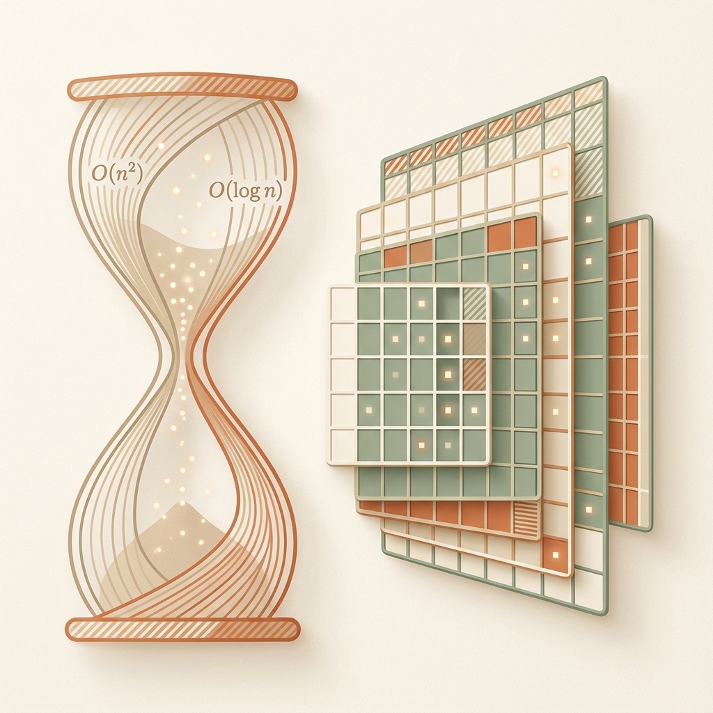
Often, you can make your code run faster by using more memory. In coding interviews, this is a very common trick.
- Can you solve a two-sum problem in
O(n)instead ofO(n^2)? Yes, by using a hash map (O(n)space complexity) to store seen numbers. - Can you traverse a tree iteratively instead of recursively? Yes, which often saves stack frame space.
Practical Tips for Your Next Technical Interview
- Drop the Constants:
O(2n)simplifies toO(n).O(n^2 + 50n)simplifies toO(n^2). Always focus on the dominant term. - Talk Through the Trade-offs: Don't just give the answer. Tell the interviewer: "I could write this with
O(1)auxiliary space, but it would takeO(n^2)time. Instead, if I useO(n)memory with a Hash Set, I can reduce the runtime toO(n)." This shows you understand engineering realities. - Practice on Realistic Platforms: The best way to get comfortable with these concepts is by writing real code and seeing how it evaluates. Using platforms like totop.app lets you practice common patterns, run mock interviews, and get immediate feedback on correctness and performance.
Understanding Big-O isn't about memorizing math formulas; it's about building an intuition for how code behaves at scale. Next time you write a nested loop, pause and ask yourself: Is there a way to solve this using a map or binary search instead? Your future servers (and your interviewer) will thank you.
Practice Full Stack Engineer Questions Live with AI Mock Interviews
Turn any job description across Engineering, DevOps, Data, Marketing, Sales, Finance, or HR into a personalized test and live voice or text AI mock interview on totop.app, or test your speed right now in the 60-Second Full Stack Engineer Blitz.
Play 60s Full Stack Engineer Blitz (Free, No Login) | Start 14-Day Free Trial | Browse All Interview Guides